What Claude-Generated Diagrams Actually Look Like Across Four Tools

The previous post covers the toolchain. This one is about using Claude to generate the actual diagram source, what that process looked like, and what the rendered outputs are.

The short version: Claude generates syntactically correct diagram code reliably. The quality of what it generates, meaning whether the layout is readable, whether the annotations are accurate, whether the diagram actually communicates the concept, varies a lot by tool and by subject.

How the generation worked

For each diagram I gave Claude the subject and the tool. For ML algorithm diagrams (CNN, SVM, Viterbi, backpropagation) I also gave the mathematical context. For infrastructure diagrams I described the architecture.

Claude produced complete source files. I fed them to the renderer, looked at the output, and iterated. Most diagrams took two or three rounds. A few took more. The Pikchr SVM diagram, which required placing scatter points at specific coordinates with a diagonal hyperplane at the right angle, took the most back-and-forth, because Pikchr requires exact geometry and there is no layout engine to fall back on.

VGG-16 Convolutional Neural Network

The CNN architecture is a natural fit for Graphviz. It is a pure DAG, one direction, layered blocks, no geometry needed. Claude generated a clean DOT file on the first try. The subgraph clusters map directly onto conv blocks, parameter counts go in the labels, and the dot engine handles all placement.

VGG-16 CNN — Graphviz — VGG-16 architecture, Graphviz dot. Five conv blocks plus classifier head.

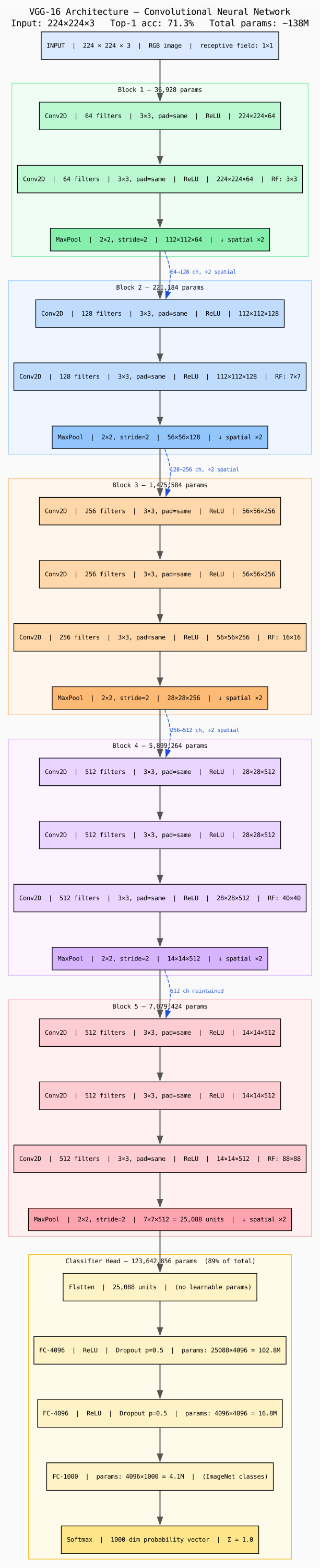
The parameter counts in the labels are accurate. Claude computed them correctly, including the receptive field annotations at each block boundary. This is the kind of detail where a human drawing the same diagram by hand would likely skip or round.

The D2 version of the same diagram is more verbose but renders well. The Mermaid and Pikchr versions exist too. None of them add information the Graphviz version does not have. For a pure DAG like this, Graphviz is the right tool and produces the cleanest result.

Support Vector Machine

The SVM diagram is where the tool choice matters most. The diagram needs a diagonal hyperplane at a specific angle, scatter points in two classes positioned relative to the hyperplane, support vectors annotated, margin width indicated with a two-headed arrow, and reference boxes for the optimisation objective and kernels. That is a geometric drawing problem.

SVM — Pikchr — SVM geometry, Pikchr. Axes, scatter plot, hyperplane at exact angle, margin annotation.

Claude handled the Pikchr geometry correctly after a couple of iterations. The initial version had the hyperplane at the wrong slope and the scatter points too tightly clustered. After adjusting the endpoint coordinates for the hyperplane line and spreading the class distributions, the diagram reads correctly.

The Graphviz SVM version uses neato with pinned pos= coordinates to approximate the same layout. It works, but you can see it fighting the tool. Pikchr is simply the right choice for this kind of figure.

Viterbi Algorithm

The Viterbi trellis is a grid: states as rows, time steps as columns, transition edges between every state pair at each step, with the optimal path highlighted. Graphviz handles this well with rankdir=LR and explicit rank=same groupings.

Viterbi trellis — Graphviz — Viterbi algorithm over 6 time steps, Graphviz dot. Optimal path in red. Delta probabilities and emission values annotated per cell.

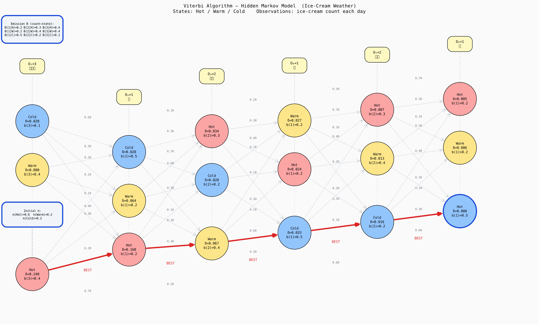
The delta values at each trellis cell are correct. Claude computed them step by step using the HMM parameters. The optimal path (H H W C C C) matches what you get running the algorithm by hand.

One thing Claude did well here: the observation nodes are tied to each column using rank=same, which keeps the column structure readable even with all the crossing transition edges. That is a non-obvious Graphviz trick.

Backpropagation

The backprop diagram is dense. Forward pass edges go left to right in blue, backward pass edges go right to left in red dashed. Every layer is fully connected to the next, so the edge count is high.

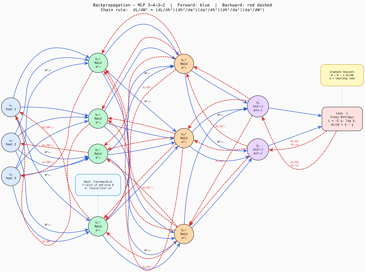
This one required the most iteration on layout. With constraint=false on the backward edges, the engine tries to route them without affecting the forward-pass layout, but on a dense fully-connected graph the result is still visually noisy. The key gradient labels (∂L/∂W¹₁₁ etc.) are annotated on representative edges only, not all of them.

Hidden Markov Model structure

The HMM diagram is the model itself, not the algorithm run on it. Hidden states with transition probabilities (including self-loops), emission probabilities to observation nodes, and initial distribution.

HMM — Graphviz — HMM structure, Graphviz dot. Transition edges blue, emission edges orange dashed.

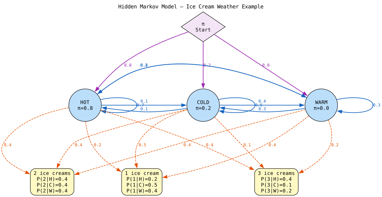
The self-loops (H→H, C→C, W→W) render cleanly in Graphviz. Most other tools handle self-loops poorly or not at all. This is one area where DOT’s maturity shows.

ML training pipeline

For an end-to-end pipeline with a feedback loop, D2 with ELK produces a cleaner result than Graphviz. The retrain trigger edge from monitoring back to ingestion crosses several other elements, and ELK routes it without collisions.

The nested training container with epochs and checkpoints inside it renders cleanly in D2. Graphviz could do this with subgraphs but the ELK routing handles the backward retrain edge better.

Transformer architecture

The transformer encoder-decoder has enough nested structure (six-layer encoder, six-layer decoder, cross-attention connecting them) that D2’s container model is a natural fit.

Transformer — D2 — Transformer encoder-decoder, D2 with ELK. Encoder K,V feed into decoder cross-attention.

Microservices architecture

The same architecture drawn in both D2 and Mermaid. D2 with ELK routes the dense cross-layer edges more cleanly. Mermaid’s dagre lays it out more compactly but the edge routing gets crowded in the middle.

Microservices — D2 — ML platform microservices, D2 with ELK.

Microservices — Mermaid — Same architecture, Mermaid with dagre. More compact but edge routing is denser.

Mermaid won on this particular diagram for use in a blog post. The output is more compact and fits the page width better. D2’s ELK layout produces a taller diagram that requires more scrolling.

ML training loop sequence

Sequence diagrams with loop and alt blocks are Mermaid’s strongest feature. The D2 version of the same diagram annotates the loop semantics on individual messages instead, because those constructs do not exist in D2’s sequence syntax.

ML training loop — Mermaid — Training loop sequence diagram, Mermaid. loop and alt are native constructs.

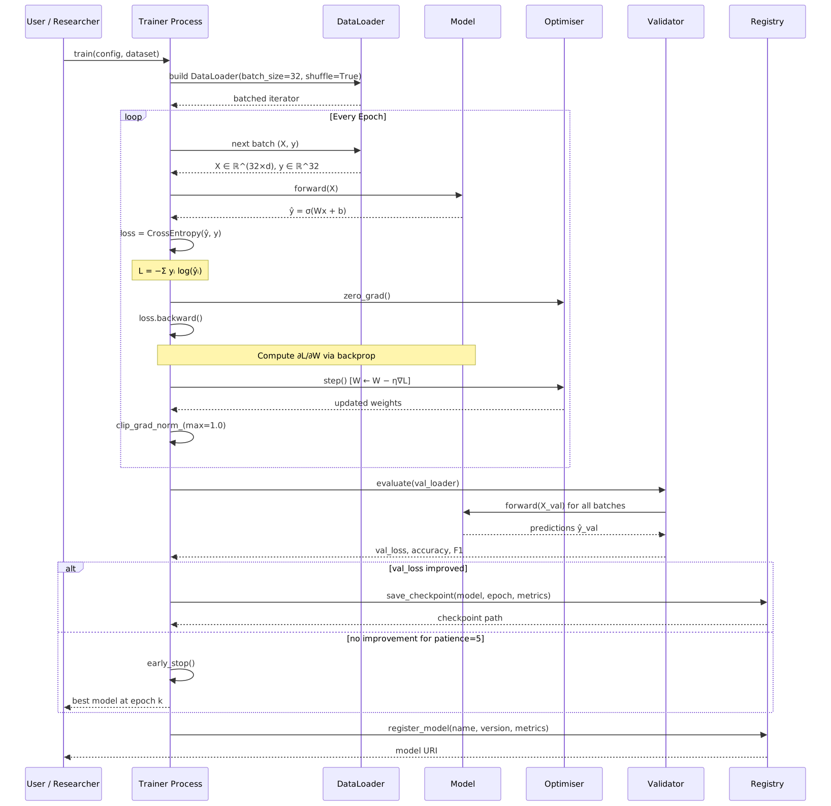
Gradient descent flowchart

Gradient descent — Mermaid — Gradient descent with scheduler branching and convergence check, Mermaid.

Kalman filter

The Kalman predict-update cycle is a two-box diagram with input arrows and a feedback loop. Pikchr handles it cleanly with named box anchors and the then left until even with arrow routing syntax.

Decision tree

What held up and what did not

Claude generated syntactically correct code for all four tools without exception. The accuracy of the mathematical content (parameter counts, probability values, gradient expressions) was consistently correct and would have taken significant time to write by hand.

The failure modes were layout-related, not content-related. Pikchr requires knowing the exact coordinates you want before you start. Claude’s initial coordinate estimates for the SVM scatter plot put the hyperplane at the wrong angle and the support vectors too close to the margin. Fixing it meant specifying the endpoint coordinates explicitly and iterating.

For graph tools, Claude sometimes generated too many label edges on dense graphs, making the result unreadable. The solution was to label only representative edges, not every one.

The Pikchr backprop diagram does not exist in this set. Pikchr can draw it (circles at coordinates, arrows between them) but the result would be manually placing every neuron and every edge. For a fully-connected network that is around 150 arrows. Claude can generate that but it is not a good use of Pikchr. The Graphviz version is better for that specific diagram.